Decentralized Joint Control

The equation of motion of a manipulator without end-effector contact force and any joint friction is

\[\label{equ.dyn} \boldsymbol{B}(\boldsymbol{q}) \ddot{\boldsymbol{q}}+\boldsymbol{C}(\boldsymbol{q}, \dot{\boldsymbol{q}}) \dot{\boldsymbol{q}}+\boldsymbol{g}(\boldsymbol{q})=\boldsymbol{\tau}\]

Let \(\boldsymbol{q}_{m}=[\theta_{m1}, \theta_{m2}, ...\theta_{mn}]^T\) denote the vector of all corresponding DM motor angles. The transmissions establish a relationship:

\[\label{equ.motor_angle} \boldsymbol{K}_{r} \boldsymbol{q}=\boldsymbol{q}_{m}\]

where \(\boldsymbol{K}_{r}=\text{diag}(k_{r_1}, k_{r_2}, ..., k_{r_n})\) is a diagonal matrix, and each diagonal element \(k_{r_i}\) is the gear ratio of joint \(i\). Let \(\boldsymbol{\tau}_{m}=[\tau_{m1},\tau_{m2},...,,\tau_{mn}]^T\) denote the vector of all motor torques, one can write

\[\label{equ.motor_torque} \boldsymbol{\tau}_{m}=\boldsymbol{K}_{r}^{-1} \boldsymbol{\tau}\]

Substituting ([equ.motor_angle]{reference-type=”ref” reference=”equ.motor_angle”}) and ([equ.motor_torque]{reference-type=”ref” reference=”equ.motor_torque”}) into the manipulator dynamics ([equ.dyn]{reference-type=”ref” reference=”equ.dyn”}) leads to

\[\label{equ.dyn2} \boldsymbol{K}_{r}^{-1} \boldsymbol{B}(\boldsymbol{q}) \boldsymbol{K}_{r}^{-1} \ddot{\boldsymbol{q}}_{m}+\boldsymbol{K}_{r}^{-1} \boldsymbol{C}(\boldsymbol{q}, \dot{\boldsymbol{q}}) \boldsymbol{K}_{r}^{-1} \dot{\boldsymbol{q}}_{m}+\boldsymbol{K}_{r}^{-1} \boldsymbol{g}(\boldsymbol{q})=\boldsymbol{\tau}_{m}\]

We have previously analyzed elements in matrix \(\boldsymbol{B}(\boldsymbol{q})\), one can write it as

\[\label{equ.bmat} \boldsymbol{B}(\boldsymbol{q})=\overline{\boldsymbol{B}}+\Delta \boldsymbol{B}(\boldsymbol{q}) \]

where \(\overline{\boldsymbol{B}}\) is the diagonal matrix whose constant elements represent the average inertia at each joint, and elements in \(\Delta \boldsymbol{B}(\boldsymbol{q})\) represent the matrix of non-diagonal part. Substituting ([equ.bmat]{reference-type=”ref” reference=”equ.bmat”}) into ([equ.dyn2]{reference-type=”ref” reference=”equ.dyn2”}) leads to

\[\label{equ.decouple_model} \underbrace{\boldsymbol{K}_{r}^{-1} \overline{\boldsymbol{B}} \boldsymbol{K}_{r}^{-1}}_{\boldsymbol{I}_m} \ddot{\boldsymbol{q}}_{m}+\underbrace{\boldsymbol{K}_{r}^{-1} \Delta \boldsymbol{B}(\boldsymbol{q}) \boldsymbol{K}_{r}^{-1} \ddot{\boldsymbol{q}}_{m}+\boldsymbol{K}_{r}^{-1} \boldsymbol{C}(\boldsymbol{q}, \dot{\boldsymbol{q}}) \boldsymbol{K}_{r}^{-1} \dot{\boldsymbol{q}}_{m}+\boldsymbol{K}_{r}^{-1} \boldsymbol{g}(\boldsymbol{q})}_{\boldsymbol{D}}=\boldsymbol{\tau}_{m}\]

The above equation ([equ.decouple_model]{reference-type=”ref” reference=”equ.decouple_model”}) will lead to the following diagram.

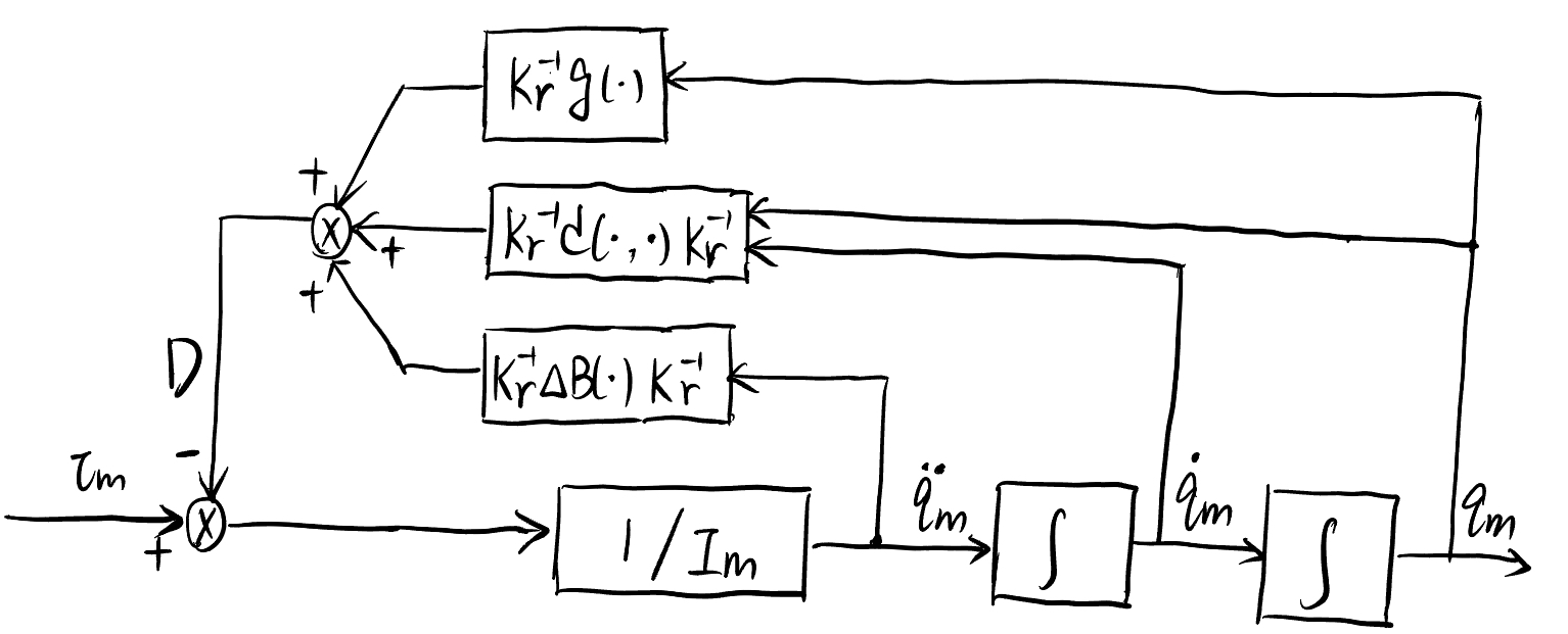
Fig. 71 Dynamics diagram of a motor-driven manipulator.

As shown in Fig. 1{reference-type=”ref” reference=”fig:3”} and ([equ.decouple_model]{reference-type=”ref” reference=”equ.decouple_model”}), if we don’t consider \(\boldsymbol{D}\), then

\[\boldsymbol{I}_m\boldsymbol{\ddot{q}}_m=\boldsymbol{\tau}_m,\]

Note that in the above equation \(\boldsymbol{I}_m\) is also a diagonal matrix. This means that if we don’t consider the complex \(\boldsymbol{D}\), each joint is a single-in-single-output system:

\[\label{equ.single_joint_dyn} {I}_m{\ddot{\theta}_m}=\tau_m\]

for each joint motor and we can control each joint individually. However, \(\boldsymbol{D}\) in ([equ.decouple_model]{reference-type=”ref” reference=”equ.decouple_model”}) is a coupling term that prevents us from doing so. To address such, in the following, we still consider the control each joint as a single-in-single-out system, but consider \(\boldsymbol{D}\) as a disturbance to each joint.

Single-Joint Control Diagram

For each joint (we omit the joint index \(i\) below), considering ([equ.single_joint_dyn]{reference-type=”ref” reference=”equ.single_joint_dyn”}) and the motor model in the previous lecture (Lecture 19), we have

\[\label{equ.motor} I_m\ddot{\theta}_m+D=\tau_m=I_m\ddot{\theta}_m+\frac{k_t}{R_a}(\frac{DR_a}{k_t})=\tau_m=k_ti_a=k_t\frac{(v_a-k_v\dot{\theta}_m)}{R_a}=k_t\frac{(G_vv_c-k_v\dot{\theta}_m)}{R_a} \]

Here, \(D\) is the disturbance torque in ([equ.decouple_model]{reference-type=”ref” reference=”equ.decouple_model”}) applied to each joint, \({k}_{t}\) is the torque constants; \({i}_{a}\) is the armature current; \({v}_{a}\) is the vector of armature voltage; \({R}_{a}\) is the armature resistance; \({k}_{v}\) is the back EMF constant; \(\boldsymbol{v}_{c}\) is the voltage of the servomotor, and \(G_v\) is amplifier. Those motor parameters have been shown in previous lecture. In the following, we will suppose \(v_c=v_a\), i.e., \(G_v=1\), for notation simplicity, and so we will directly treat \(v_a\) as the servo motor input voltage. But the analysis also holds for any \(G_v\).

The above ([equ.motor]{reference-type=”ref” reference=”equ.motor”}) corresponds to the following diagram:

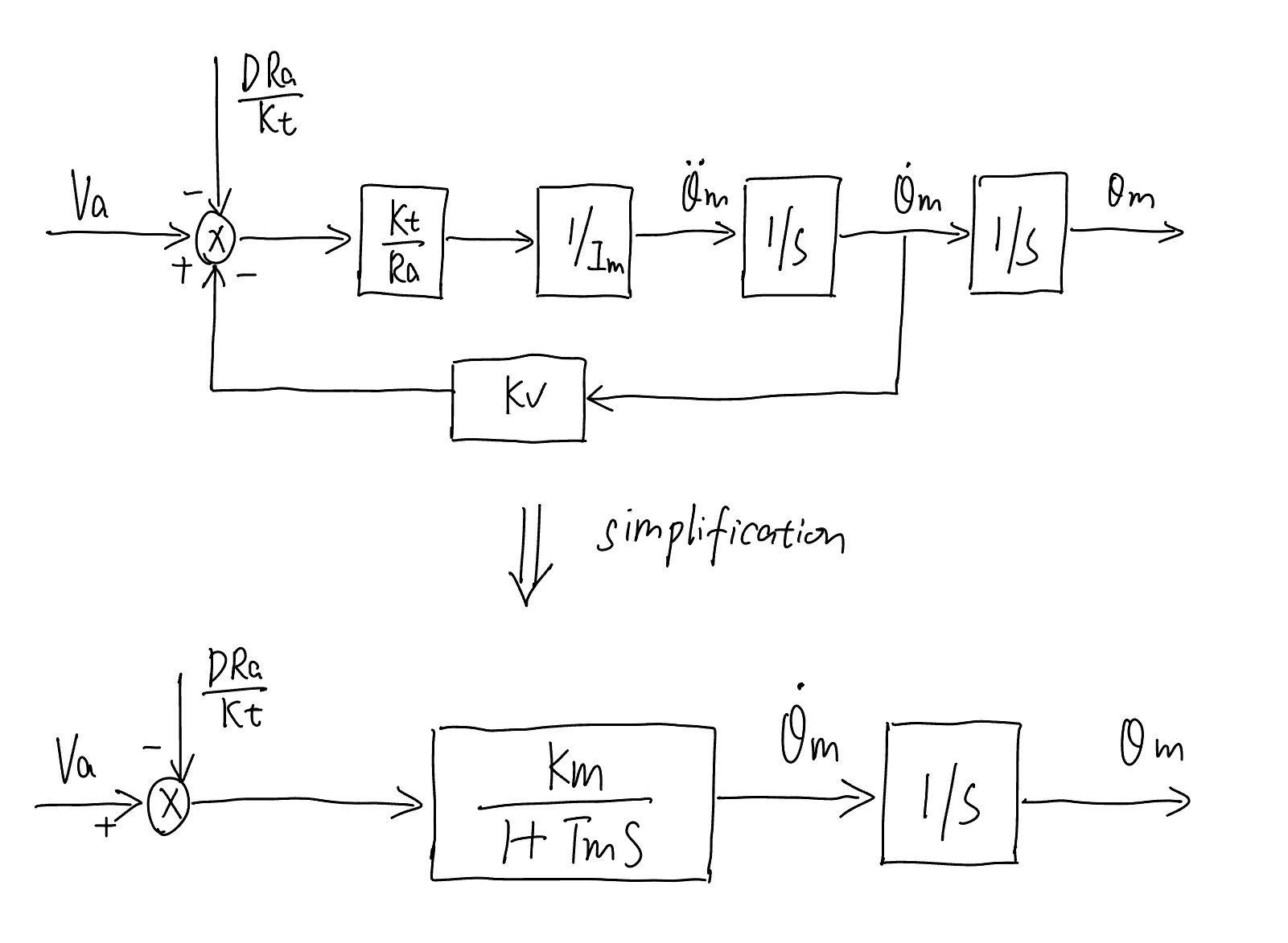
Fig. 72 Diagram of a motor-driven manipulator, with coupled joint terms treated as disturbance.

In the above diagram, the closed loop is due to the DC motor model itself. We write input (\(V_a\)) to output (\(\theta_m\)) transfer function $\(\label{equ.motortf} G(s)=\frac{{\Theta}(s)}{V_a(s)}=\frac{k_m}{s(1+T_ms)}\)$

\[\frac{\dot{\Theta}(s)}{V_a(s)}=\frac{\frac{k_t}{R_aI_ms}}{1+\frac{k_t}{R_aI_ms}k_v}=\frac{k_m}{1+T_ms}\]

Minimal Control Background

For ease of the reader, we provide the following minimal background of control design. A typical closed-loop control diagram is shown below. Here, \(\theta_r\) is the reference input; \(\theta_m\) is the output; \(D\) is the disturbance; \(G(s)\) is the transfer function of the plant to be controlled; \(C(s)\) is the controller; \(H(s)\) is the backward pass transfer function (usually a constant due to sensor). The goal of control design is to find \(C(s)\) such that \(\theta_m\) is able to track \(\theta_r\) while \(D\) has as little effect on \(\theta_m\) as possible.

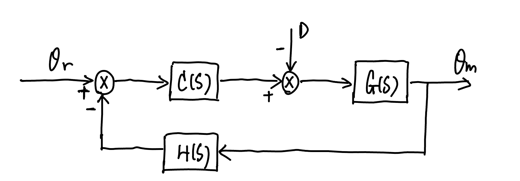
Fig. 73 A typical control system diagram

For the above control system, the forward path transfer function is

\[P(s)=C(s)G(s)\]

The backward path transfer function is $\(H(s)\)$ The open loop transfer function is

\[C(s)G(s)H(s)\]

The input-to-output transfer function is

\[ \frac{\Theta_m(s)}{\Theta_r(s)}=\frac{C(s)G(s)}{1+C(s)G(s)H(s)} \]

The disturbance-to-output transfer function is

\[ \frac{\Theta_m(s)}{D(s)}=\frac{G(s)}{1+C(s)G(s)H(s)} \]

The input (\(\theta_r\)) to output (\(\theta_m\)) response of the closed-loop system will be determined by the roots of the characteristics equation $\(1+C(s)G(s)H(s)=0\)$

Background of final value theorem

If a continuous signal \(f(t)\) has its Laplace transformation \(F(s)\), then the final value theorem states

\[\lim_{t\rightarrow\infty}f(t)=\lim_{s\rightarrow 0}sF(s)\]

Single Joint Position feedback

The single joint motor system in Fig 2{reference-type=”ref” reference=”fig:motor_model2”} is the plant we want to control. The plant transfer function \(G(s)\) is ([equ.motortf]{reference-type=”ref” reference=”equ.motortf”}), rewritten below

\[G(s)=\frac{k_m}{s(1+T_ms)}\]

We want to design a proportional-integral controller

\[\begin{gathered} C_{P}(s)=K_{P} \frac{1+s T_{P}}{s} \end{gathered}\]

with \(K_P\) and \(T_P\) are design variable.

The control diagram thus is shown below (note that the backward pass constant \(k_{TP}\) is fixed).

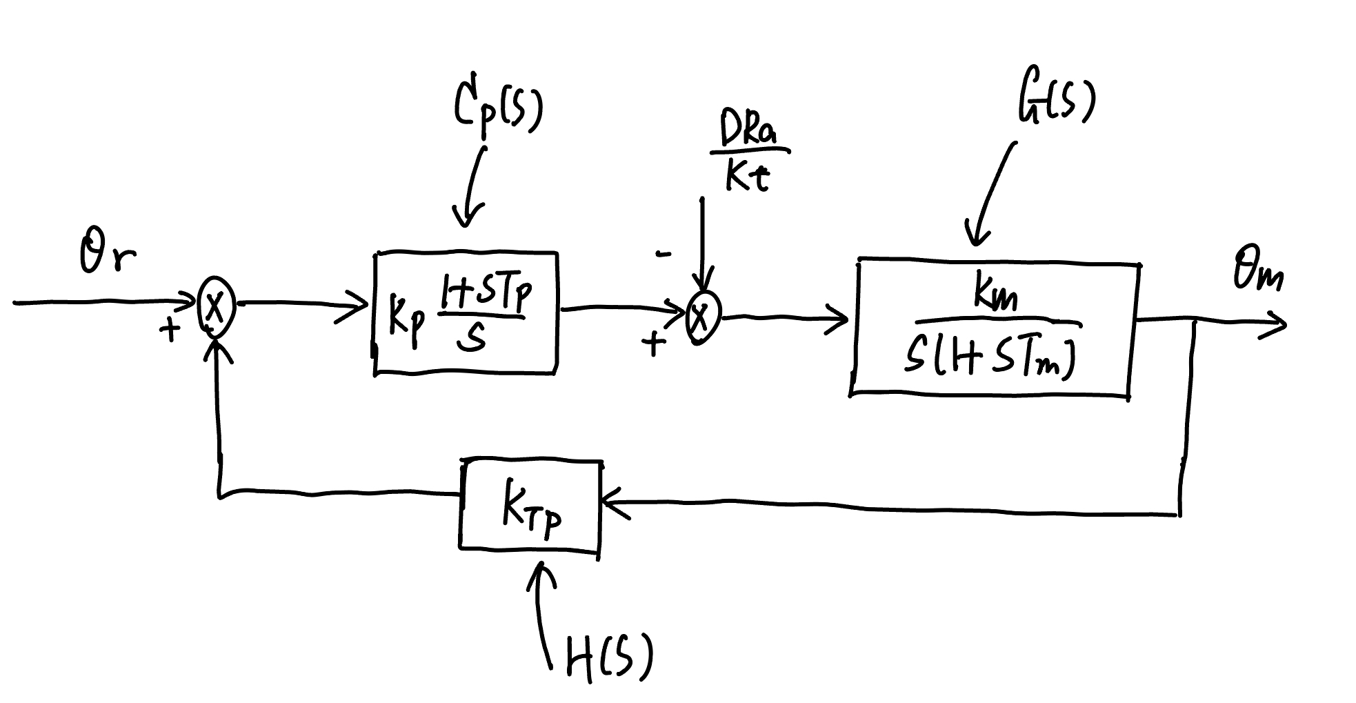
Fig. 74 Control diagram of position decentralized joint space control

The transfer function of the forward path is

\[P(s)=G(s)C_P(s)=\frac{k_{m} K_{P}\left(1+s T_{P}\right)}{s^{2}\left(1+s T_{m}\right)}\]

The transfer function of the backward pass is

\[H(s)=k_{T P}\]

The root locus can be plotted as a function of the gain of the position loop \(k_{m} K_{P} k_{T P} T_{P} / T_{m}\). Here, we derive into two cases to plot the root locus.

• If \(T_{P}<T_{m}\), the root locus is shown as below. Thus, the system is inherently unstable.

  

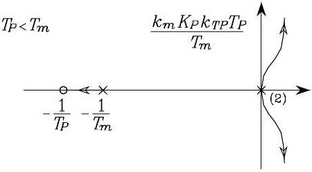
  Fig. 75 Root locus when \(T_{P}<T_{m}\)

• If \(T_{P}>T_{m}\), the root locus is shown as below. As \(T_{P}\) increases, the absolute value of the real part of the two roots of the locus tending towards the asymptotes increases too, and the system has faster time response.

  

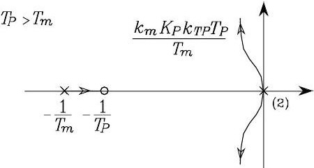
  Fig. 76 Root locus when \(T_{P}>T_{m}\)

The closed-loop input/output transfer function is

\[\frac{\Theta_{m}(s)}{\Theta_{r}(s)}=\frac{P(s)}{1+P(s)H(s)}=\frac{{k_{m}K_P(1+T_Ps)}}{k_{TP}k_{m}K_P(1+T_Ps)+s^2(1+sT_m)},\]

and the characteristic equation can be factorized into the following form

\[{k_{TP}k_{m}K_P(1+T_Ps)+s^2(1+sT_m)} = {\left({\omega_{n}^{2}}+{2 \zeta }{\omega_{n}}s+{s^{2}}\right)(1+s \tau)}\]

where \(\omega_{n}\) and \(\zeta\) are the natural frequency and damping ratio of the complex poles: \(\left(-\zeta \omega_{n}, \pm j \sqrt{1-\zeta^{2}} \omega_{n}\right)\), and \(-1 / \tau\) is the real pole. These poles correspond to the ones in the root locus in the above figures.

The closed-loop disturbance/output transfer function is

\[\frac{\Theta_{m}(s)}{D(s)}=-\frac{\frac{R_a}{K_t}G(s)}{1+P(s)H(s)}=-\frac{\frac{R_a}{K_t}k_ms}{k_{TP}k_{m}K_P(1+T_Ps)+s^2(1+sT_m)}\]

If \(\Theta_r(t)=0\), based on the final value theory, we have

\[\lim_{t\rightarrow \infty} {\theta_{m}(t)}= \lim_{s\rightarrow 0} s{\Theta_{m}(s)}=\lim_{s\rightarrow 0} s\frac{\Theta_{m}(s)}{D(s)}{D(s)}\]

thus,

\[\begin{split}\lim_{t\rightarrow \infty} {\theta_{m}(t)}= \begin{cases} 0\qquad &\text{if}\quad D(t)\,\,\text{is constant signal}\\ \frac{R_a}{K_t}\frac{1}{K_{P} k_{T P}} \qquad &\text{if}\quad D(t)\,\,\text{is ramp signal, such as $D(t)=vt$ }\\ \end{cases}\end{split}\]

Hence, the controller can cancel the effect of constant disturbance, and the quantity

\[K_{P} k_{T P}\]

can be interpreted as the disturbance rejection factor for velocity (or higher-order) disturbance. Increasing \(K_{P}\) can help with reducing the effect of \(D\), but too high \(K_P\) can lead to unacceptable oscillations of the output, as implied from the root locus.

Single-Joint Position and Velocity Feedback

To control the motor system in Fig. 2{reference-type=”ref” reference=”fig:motor_model2”}, we use both position and velocity controller $\(\begin{gathered} C_{P}(s)=K_{P} \quad \text{and} \quad C_{V}(s)=K_{V} \frac{1+s T_{V}}{s} \end{gathered}\)\( where \)K_p\(, \)K_v\(, and \)T_v$ are the design variables.

The control diagram is shown below (Note that \(k_{TV}\) and \(k_{TP}\) in the backward pass are fixed).

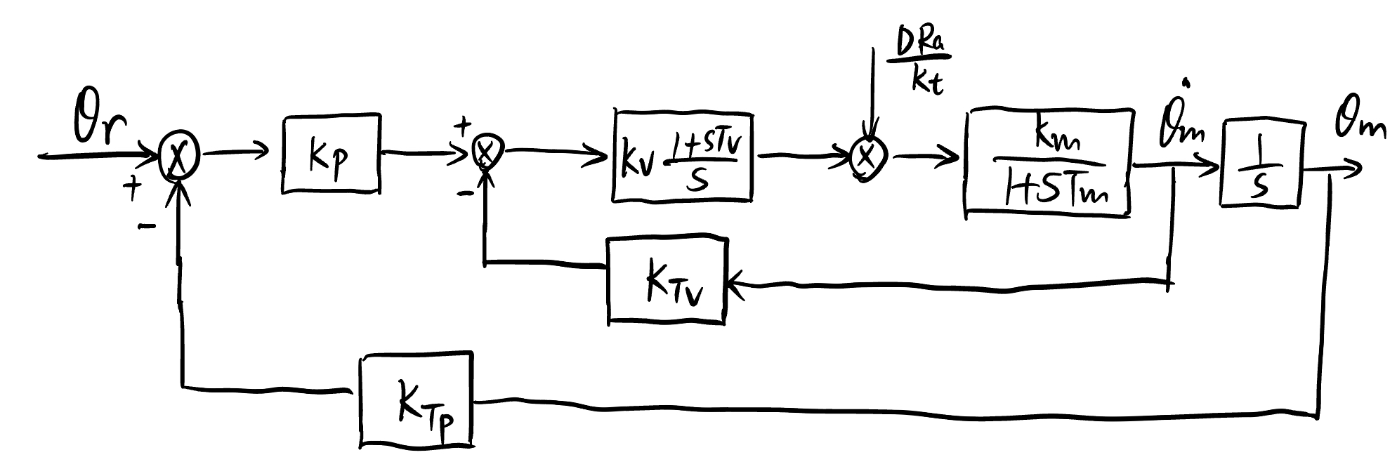
Fig. 77 Control diagram of position and velocity control

which can be further reduced into the following diagram:

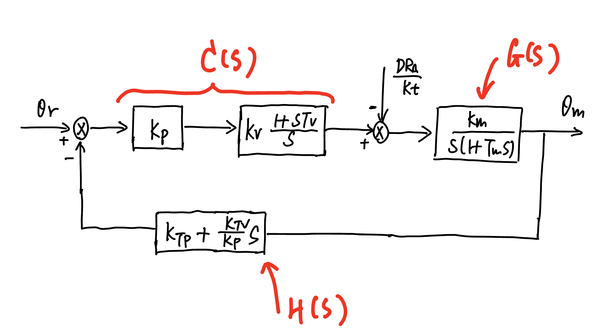
Fig. 78 Corresponding to Fig. 7{reference-type=”ref” reference=”fig.pv_control”}, the equivalent control diagram

The transfer function of the forward path is

\[P(s)=C(s)G(s)=\frac{k_{m} K_{P} K_{V}\left(1+s T_{V}\right)}{s^{2}\left(1+s T_{m}\right)}\]

The transfer function of the backward path is

\[H(s)=k_{T P}\left(1+s \frac{k_{T V}}{K_{P} k_{T P}}\right) .\]

For simplicity, one can design

\[T_m=T_v,\]

then that the poles of the closed-loop system move on the root locus as a function of the loop gain \(k_{m} K_{V} k_{T V}\) is shown in the following figure:

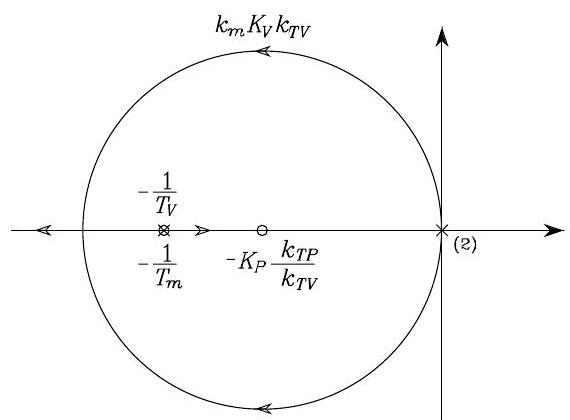
Fig. 79 Root locus

By increasing the position gain \(K_{P}\), it is possible to confine the closed-loop poles into a region of the complex plane with large absolute values of the real part.

The closed-loop input/output transfer function is

\[\frac{\Theta_{m}(s)}{\Theta_{r}(s)}=\frac{C(s)G(s)}{1+C(s)G(s)H(s)}=\frac{\frac{1}{k_{T P}}}{1+\frac{s k_{T V}}{K_{P} k_{T P}}+\frac{s^{2}}{k_{m} K_{P} k_{T P} K_{V}}}=\frac{\frac{1}{k_{T P}}}{1+\frac{2 \zeta s}{\omega_{n}}+\frac{s^{2}}{\omega_{n}^{2}}}\]

It can be recognized that, with a suitable choice of the gains, it is possible to obtain any value of natural frequency \(\omega_{n}\) and damping ratio \(\zeta\). Hence, if \(\omega_{n}\) and \(\zeta\) are given as design requirements, the following relations is

\[K_{V} k_{T V}=\frac{2 \zeta \omega_{n}}{k_{m}}\]

\[K_{P} k_{T P} K_{V}=\frac{\omega_{n}^{2}}{k_{m}}\]

For given transducer constants \(k_{T P}\) and \(k_{T V}\), \(K_{V}\) and \(K_{P}\) can be chosen. The closed-loop disturbance/output transfer function is

\[\frac{\Theta_{m}(s)}{D(s)}=-\frac{\frac{R_a}{k_t}G(s)}{1+P(s)H(s)}=-\frac{\frac{R_a}{k_t}k_ms}{(1+sT_m)(s^2+k_mK_Vk_{TV}s+k_mK_PK_Vk_{TP})}\]

which shows that the disturbance rejection factor is

If \(\Theta_r(t)=0\), based on the final value theory, we have

\[\lim_{t\rightarrow \infty} {\theta_{m}(t)}= \lim_{s\rightarrow 0} s{\Theta_{m}(s)}=\lim_{s\rightarrow 0} s\frac{\Theta_{m}(s)}{D(s)}{D(s)}\]

thus,

\[\begin{split}\lim_{t\rightarrow \infty} {\theta_{m}(t)}= \begin{cases} 0\qquad &\text{if}\quad D(t)\,\,\text{is constant signal}\\ \frac{R_a}{k_t}\frac{1}{K_{P} k_{T P} K_{V}} \qquad &\text{if}\quad D(t)\,\,\text{is ramp signal, such as $D(t)=vt$ }\\ \end{cases}\end{split}\]

Hence, the controller can cancel the effect of constant disturbance, and the quantity

\[K_{P} k_{T P} K_{V}\]

can be interpreted as the disturbance rejection factor for velocity (or higher-order) disturbance. Increasing \(K_{P}\) and \(K_V\) can help with reducing the effect of \(D\).